The RPython Toolchain
Contents
This document describes the toolchain that we have developed to analyze and “compile” RPython programs (like PyPy itself) to various target platforms.
It consists of three broad sections: a slightly simplified overview, a brief introduction to each of the major components of our toolchain and then a more comprehensive section describing how the pieces fit together. If you are reading this document for the first time, the Overview is likely to be most useful, if you are trying to refresh your PyPy memory then the How It Fits Together is probably what you want.
Overview
The job of the translation toolchain is to translate RPython programs into an efficient version of that program for one of various target platforms, generally one that is considerably lower-level than Python. It divides this task into several steps, and the purpose of this document is to introduce them.
To start with we describe the process of translating an RPython program into C (which is the default and original target).
The RPython translation toolchain never sees Python source code or syntax trees, but rather starts with the code objects that define the behaviour of the function objects one gives it as input. The flow graph builder works through these code objects using abstract interpretation to produce a control flow graph (one per function): yet another representation of the source program, but one which is suitable for applying type inference and translation techniques and which is the fundamental data structure most of the translation steps operate on.
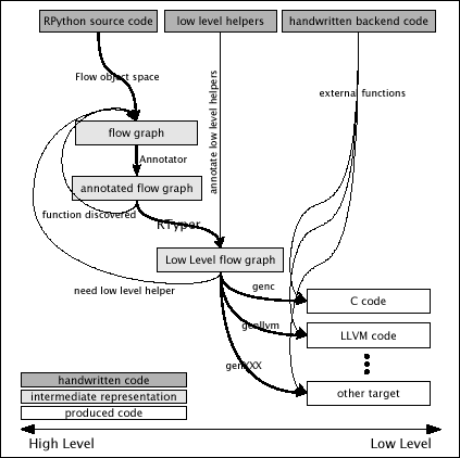
It is helpful to consider translation as being made up of the following steps (see also the figure below):
- The complete program is imported, at which time arbitrary run-time initialization can be performed. Once this is done, the program must be present in memory as a form that is “static enough” in the sense of RPython.
- The Annotator performs a global analysis starting from a specified entry point to deduce type and other information about what each variable can contain at run-time, building flow graphs as it encounters them.
- The RPython Typer (or RTyper) uses the high-level information inferred by the Annotator to turn the operations in the control flow graphs into low-level operations.
- After the RTyper there are several optional optimizations which can be applied and are intended to make the resulting program go faster.
- The next step is preparing the graphs for source generation, which involves computing the names that the various functions and types in the program will have in the final source and applying transformations which insert explicit exception handling and memory management operations.
- The C backend (colloquially known as “GenC”) produces a number of C source files (as noted above, we are ignoring the other backends for now).
- These source files are compiled to produce an executable.
(although these steps are not quite as distinct as you might think from this presentation).
There is an interactive interface called rpython/bin/translatorshell.py to the translation process which allows you to interactively work through these stages.
The following figure gives a simplified overview (PDF color version):
Building Flow Graphs
Introduction
The task of the flow graph builder (the source is at rpython/flowspace/) is to generate a control-flow graph from a function. This graph will also contain a trace of the individual operations, so that it is actually just an alternate representation for the function.
The basic idea is that if an interpreter is given a function, e.g.:
def f(n):
  return 3*n+2
it will compile it to bytecode and then execute it on its VM. Instead, the flow graph builder contains an abstract interpreter which takes the bytecode and performs whatever stack-shuffling and variable juggling is needed, but merely records any actual operation performed on a Python object into a structure called a basic block. The result of the operation is represented by a placeholder value that can appear in further operations.
For example, if the placeholder v1 is given as the argument to the above
function, the bytecode interpreter will call v2 = space.mul(space.wrap(3),
v1) and then v3 = space.add(v2, space.wrap(2)) and return v3 as the
result. During these calls, the following block is recorded:
Block(v1):     # input argument
  v2 = mul(Constant(3), v1)
  v3 = add(v2, Constant(2))
Abstract interpretation
build_flow() works by recording all operations issued by the bytecode
interpreter into basic blocks. A basic block ends in one of two cases: when
the bytecode interpreters calls is_true(), or when a joinpoint is reached.
- A joinpoint occurs when the next operation is about to be recorded into the current block, but there is already another block that records an operation for the same bytecode position. This means that the bytecode interpreter has closed a loop and is interpreting already-seen code again. In this situation, we interrupt the bytecode interpreter and we make a link from the end of the current block back to the previous block, thus closing the loop in the flow graph as well. (Note that this occurs only when an operation is about to be recorded, which allows some amount of constant-folding.)
- If the bytecode interpreter calls
is_true(), the abstract interpreter doesn’t generally know if the answer should be True or False, so it puts a conditional jump and generates two successor blocks for the current basic block. There is some trickery involved so that the bytecode interpreter is fooled into thinking thatis_true()first returns False (and the subsequent operations are recorded in the first successor block), and later the same call tois_true()also returns True (and the subsequent operations go this time to the other successor block).
(This section to be extended…)
The Flow Model
Here we describe the data structures produced by build_flow(), which are
the basic data structures of the translation process.
All these types are defined in rpython/flowspace/model.py (which is a rather important module in the PyPy source base, to reinforce the point).
The flow graph of a function is represented by the class FunctionGraph.
It contains a reference to a collection of Blocks connected by Links.
A Block contains a list of SpaceOperations. Each SpaceOperation
has an opname and a list of args and result, which are either
Variables or Constants.
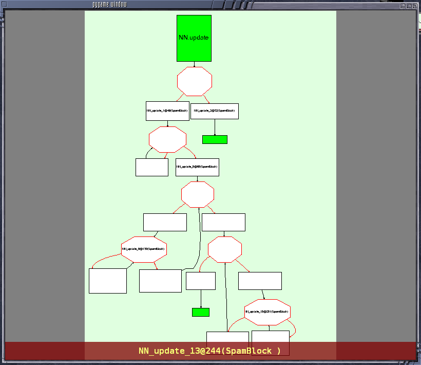
We have an extremely useful PyGame viewer, which allows you to visually inspect the graphs at various stages of the translation process (very useful to try to work out why things are breaking). It looks like this:
It is recommended to play with python bin/translatorshell.py on a few
examples to get an idea of the structure of flow graphs. The following describes
the types and their attributes in some detail:
FunctionGraphA container for one graph (corresponding to one function).
startblock: the first block. It is where the control goes when the function is called. The input arguments of the startblock are the function’s arguments. If the function takes a *argsargument, theargstuple is given as the last input argument of the startblock.returnblock: the (unique) block that performs a function return. It is empty, not actually containing any returnoperation; the return is implicit. The returned value is the unique input variable of the returnblock.exceptblock: the (unique) block that raises an exception out of the function. The two input variables are the exception class and the exception value, respectively. (No other block will actually link to the exceptblock if the function does not explicitly raise exceptions.) BlockA basic block, containing a list of operations and ending in jumps to other basic blocks. All the values that are “live” during the execution of the block are stored in Variables. Each basic block uses its own distinct Variables.
inputargs: list of fresh, distinct Variables that represent all the values that can enter this block from any of the previous blocks. operations: list of SpaceOperations. exitswitch: see below exits: list of Links representing possible jumps from the end of this basic block to the beginning of other basic blocks. Each Block ends in one of the following ways:
- unconditional jump: exitswitch is None, exits contains a single Link.
- conditional jump: exitswitch is one of the Variables that appear in the Block, and exits contains one or more Links (usually 2). Each Link’s exitcase gives a concrete value. This is the equivalent of a “switch”: the control follows the Link whose exitcase matches the run-time value of the exitswitch Variable. It is a run-time error if the Variable doesn’t match any exitcase.
- exception catching: exitswitch is
Constant(last_exception). The first Link has exitcase set to None and represents the non-exceptional path. The next Links have exitcase set to a subclass of Exception, and are taken when the last operation of the basic block raises a matching exception. (Thus the basic block must not be empty, and only the last operation is protected by the handler.) - return or except: the returnblock and the exceptblock have operations set to an empty tuple, exitswitch to None, and exits empty.
LinkA link from one basic block to another.
prevblock: the Block that this Link is an exit of. target: the target Block to which this Link points to. args: a list of Variables and Constants, of the same size as the target Block’s inputargs, which gives all the values passed into the next block. (Note that each Variable used in the prevblock may appear zero, one or more times in the argslist.)exitcase: see above. last_exception: None or a Variable; see below. last_exc_value: None or a Variable; see below. Note that
argsuses Variables from the prevblock, which are matched to the target block’sinputargsby position, as in a tuple assignment or function call would do.If the link is an exception-catching one, the
last_exceptionandlast_exc_valueare set to two fresh Variables that are considered to be created when the link is entered; at run-time, they will hold the exception class and value, respectively. These two new variables can only be used in the same link’sargslist, to be passed to the next block (as usual, they may actually not appear at all, or appear several times inargs).SpaceOperationA recorded (or otherwise generated) basic operation.
opname: the name of the operation. build_flow()produces only operations from the list inrpython.flowspace.operation, but later the names can be changed arbitrarily.args: list of arguments. Each one is a Constant or a Variable seen previously in the basic block. result: a new Variable into which the result is to be stored. Note that operations usually cannot implicitly raise exceptions at run-time; so for example, code generators can assume that a
getitemoperation on a list is safe and can be performed without bound checking. The exceptions to this rule are: (1) if the operation is the last in the block, which ends withexitswitch == Constant(last_exception), then the implicit exceptions must be checked for, generated, and caught appropriately; (2) calls to other functions, as persimple_callorcall_args, can always raise whatever the called function can raise — and such exceptions must be passed through to the parent unless they are caught as above.VariableA placeholder for a run-time value. There is mostly debugging stuff here.
name: it is good style to use the Variable object itself instead of its nameattribute to reference a value, although thenameis guaranteed unique.ConstantA constant value used as argument to a SpaceOperation, or as value to pass across a Link to initialize an input Variable in the target Block.
value: the concrete value represented by this Constant. key: a hashable object representing the value. A Constant can occasionally store a mutable Python object. It represents a static, pre-initialized, read-only version of that object. The flow graph should not attempt to actually mutate such Constants.
The Annotation Pass
We describe briefly below how a control flow graph can be “annotated” to discover the types of the objects. This annotation pass is a form of type inference. It operates on the control flow graphs built by the Flow Object Space.
For a more comprehensive description of the annotation process, see the corresponding section of our EU report about translation.
The major goal of the annotator is to “annotate” each variable that appears in a flow graph. An “annotation” describes all the possible Python objects that this variable could contain at run-time, based on a whole-program analysis of all the flow graphs – one per function.
An “annotation” is an instance of a subclass of SomeObject. Each
subclass that represents a specific family of objects.
Here is an overview (see pypy/annotation/model/):
SomeObjectis the base class. An instance ofSomeObject()represents any Python object, and as such usually means that the input program was not fully RPython.SomeInteger()represents any integer.SomeInteger(nonneg=True)represent a non-negative integer (>=0).SomeString()represents any string;SomeChar()a string of length 1.SomeTuple([s1,s2,..,sn])represents a tuple of lengthn. The elements in this tuple are themselves constrained by the given list of annotations. For example,SomeTuple([SomeInteger(), SomeString()])represents a tuple with two items: an integer and a string.
The result of the annotation pass is essentially a large dictionary
mapping Variables to annotations.
All the SomeXxx instances are immutable. If the annotator needs to
revise its belief about what a Variable can contain, it does so creating a
new annotation, not mutating the existing one.
Mutable Values and Containers
Mutable objects need special treatment during annotation, because the annotation of contained values needs to be possibly updated to account for mutation operations, and consequently the annotation information reflown through the relevant parts of the flow graphs.
SomeListstands for a list of homogeneous type (i.e. all the elements of the list are represented by a single commonSomeXxxannotation).SomeDictstands for a homogeneous dictionary (i.e. all keys have the sameSomeXxxannotation, and so have all values).
User-defined Classes and Instances
SomeInstance stands for an instance of the given class or any
subclass of it. For each user-defined class seen by the annotator, we
maintain a ClassDef (pypy.annotation.classdef) describing the
attributes of the instances of the class; essentially, a ClassDef gives
the set of all class-level and instance-level attributes, and for each
one, a corresponding SomeXxx annotation.
Instance-level attributes are discovered progressively as the annotation progresses. Assignments like:
inst.attr = value
update the ClassDef of the given instance to record that the given attribute exists and can be as general as the given value.
For every attribute, the ClassDef also records all the positions where the attribute is read. If, at some later time, we discover an assignment that forces the annotation about the attribute to be generalized, then all the places that read the attribute so far are marked as invalid and the annotator will restart its analysis from there.
The distinction between instance-level and class-level attributes is
thin; class-level attributes are essentially considered as initial
values for instance-level attributes. Methods are not special in this
respect, except that they are bound to the instance (i.e. self =
SomeInstance(cls)) when considered as the initial value for the
instance.
The inheritance rules are as follows: the union of two SomeInstance
annotations is the SomeInstance of the most precise common base
class. If an attribute is considered (i.e. read or written) through a
SomeInstance of a parent class, then we assume that all subclasses
also have the same attribute, and that the same annotation applies to
them all (so code like return self.x in a method of a parent class
forces the parent class and all its subclasses to have an attribute
x, whose annotation is general enough to contain all the values that
all the subclasses might want to store in x). However, distinct
subclasses can have attributes of the same names with different,
unrelated annotations if they are not used in a general way through the
parent class.
Backend Optimizations
The point of the backend optimizations are to make the compiled program run faster. Compared to many parts of the PyPy translator, which are very unlike a traditional compiler, most of these will be fairly familiar to people who know how compilers work.
Function Inlining
To reduce the overhead of the many function calls that occur when running the
PyPy interpreter we implemented function inlining. This is an optimization
which takes a flow graph and a callsite and inserts a copy of the flow graph
into the graph of the calling function, renaming occurring variables as
appropriate. This leads to problems if the original function was surrounded by
a try: ... except: ... guard. In this case inlining is not always
possible. If the called function is not directly raising an exception (but an
exception is potentially raised by further called functions) inlining is safe,
though.
In addition we also implemented heuristics which function to inline where. For this purpose we assign every function a “size”. This size should roughly correspond to the increase in code-size which is to be expected should the function be inlined somewhere. This estimate is the sum of two numbers: for one every operations is assigned a specific weight, the default being a weight of one. Some operations are considered to be more effort than others, e.g. memory allocation and calls; others are considered to be no effort at all (casts…). The size estimate is for one the sum of the weights of all operations occurring in the graph. This is called the “static instruction count”. The other part of the size estimate of a graph is the “median execution cost”. This is again the sum of the weight of all operations in the graph, but this time weighted with a guess how often the operation is executed. To arrive at this guess we assume that at every branch we take both paths equally often, except for branches that are the end of loops, where the jump back to the end of the loop is considered more likely. This leads to a system of equations which can be solved to get approximate weights for all operations.
After the size estimate for all function has been determined, functions are being inlined into their callsites, starting from the smallest functions. Every time a function is being inlined into another function, the size of the outer function is recalculated. This is done until the remaining functions all have a size greater than a predefined limit.
Malloc Removal
Since RPython is a garbage collected language there is a lot of heap memory allocation going on all the time, which would either not occur at all in a more traditional explicitly managed language or results in an object which dies at a time known in advance and can thus be explicitly deallocated. For example a loop of the following form:
for i in range(n):
    ...
which simply iterates over all numbers from 0 to n - 1 is equivalent to the following in Python:
l = range(n)
iterator = iter(l)
try:
    while 1:
        i = iterator.next()
        ...
except StopIteration:
    pass
Which means that three memory allocations are executed: The range object, the iterator for the range object and the StopIteration instance, which ends the loop.
After a small bit of inlining all these three objects are never even passed as arguments to another function and are also not stored into a globally reachable position. In such a situation the object can be removed (since it would die anyway after the function returns) and can be replaced by its contained values.
This pattern (an allocated object never leaves the current function and thus dies after the function returns) occurs quite often, especially after some inlining has happened. Therefore we implemented an optimization which “explodes” objects and thus saves one allocation in this simple (but quite common) situation.
Escape Analysis and Stack Allocation
Another technique to reduce the memory allocation penalty is to use stack allocation for objects that can be proved not to life longer than the stack frame they have been allocated in. This proved not to really gain us any speed, so over time it was removed again.
Preparation for Source Generation
This, perhaps slightly vaguely named, stage is the most recent to appear as a separate step. Its job is to make the final implementation decisions before source generation – experience has shown that you really don’t want to be doing any thinking at the same time as actually generating source code. For the C backend, this step does three things:
- inserts explicit exception handling,
- inserts explicit memory management operations,
- decides on the names functions and types will have in the final source (this mapping of objects to names is sometimes referred to as the “low-level database”).
Making Exception Handling Explicit
RPython code is free to use exceptions in much the same way as unrestricted Python, but the final result is a C program, and C has no concept of exceptions. The exception transformer implements exception handling in a similar way to CPython: exceptions are indicated by special return values and the current exception is stored in a global data structure.
In a sense the input to the exception transformer is a program in terms of the lltypesystem with exceptions and the output is a program in terms of the bare lltypesystem.
Memory Management Details
As well as featuring exceptions, RPython is a garbage collected language; again, C is not. To square this circle, decisions about memory management must be made. In keeping with PyPy’s approach to flexibility, there is freedom to change how to do it. There are three approaches implemented today:
- reference counting (deprecated, too slow)
- using the Boehm-Demers-Weiser conservative garbage collector
- using one of our custom exact GCs implemented in RPython
Almost all application-level Python code allocates objects at a very fast rate; this means that the memory management implementation is critical to the performance of the PyPy interpreter.
A Historical Note
As this document has shown, the translation step is divided into more steps than one might at first expect. It is certainly divided into more steps than we expected when the project started; the very first version of GenC operated on the high-level flow graphs and the output of the annotator, and even the concept of the RTyper didn’t exist yet. More recently, the fact that preparing the graphs for source generation (“databasing”) and actually generating the source are best considered separately has become clear.
How It Fits Together
As should be clear by now, the translation toolchain of PyPy is a flexible and complicated beast, formed from many separate components.
digraph translation { graph [fontname = "Sans-Serif", size="6.00"] node [fontname = "Sans-Serif"] edge [fontname = "Sans-Serif"] subgraph legend { "Input or Output" [shape=ellipse, style=filled] "Transformation Step" [shape=box, style="rounded,filled"] // Invisible edge to make sure they are placed vertically "Input or Output" -> "Transformation Step" [style=invis] } "Input Program" [shape=ellipse] "Flow Analysis" [shape=box, style=rounded] "Annotator" [shape=box, style=rounded] "RTyper" [shape=box, style=rounded] "Backend Optimizations (optional)" [shape=box, style=rounded] "Exception Transformer" [shape=box, style=rounded] "GC Transformer" [shape=box, style=rounded] "GenC" [shape=box, style=rounded] "ANSI C code" [shape=ellipse] "Input Program" -> "Flow Analysis" -> "Annotator" -> "RTyper" -> "Backend Optimizations (optional)" -> "Exception Transformer" -> "GC Transformer" "RTyper" -> "Exception Transformer" [style=dotted] "GC Transformer" -> "GenC" -> "ANSI C code" // "GC Transformer" -> "GenLLVM" -> "LLVM IR" }A detail that has not yet been emphasized is the interaction of the various components. It makes for a nice presentation to say that after the annotator has finished the RTyper processes the graphs and then the exception handling is made explicit and so on, but it’s not entirely true. For example, the RTyper inserts calls to many low-level helpers which must first be annotated, and the GC transformer can use inlining (one of the backend optimizations) of some of its small helper functions to improve performance. The following picture attempts to summarize the components involved in performing each step of the default translation process:
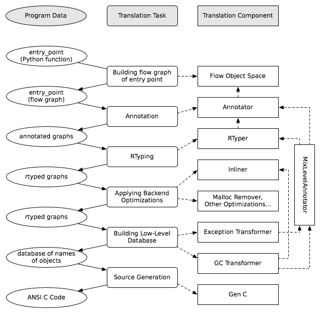
A component not mentioned before is the “MixLevelAnnotator”; it provides a convenient interface for a “late” (after RTyping) translation step to declare that it needs to be able to call each of a collection of functions (which may refer to each other in a mutually recursive fashion) and annotate and rtype them all at once.